Preprint, 11th Conf. on Num. Wea. Prediction
19-23, August 1996, Norfolk, VA
Ameri. Metero. Soc., 363-365.

PARAMETERIZATION OF PBL TURBULENCE IN A MULTI-SCALE NONHYDROSTATIC MODEL

^(1)*Ming Xue, ^(1,2)Jinxing Zong and ^(1,2) Kelvin K. Droegemeier
Center for Analysis and Prediction of Storms⁽¹⁾
School of Meteorology⁽²⁾
University of Oklahoma
Norman, OK 73019, USA

1. INTRODUCTION

Accurate prediction of daytime planetary boundary layer (PBL) evolution is very important for the prediction of warm season convection because convective storms are often initiated after a well-mixed boundary layer fully develops so as to break a pre-existing capping inversion. Unfortunately, the resolution of most numerical weather prediction (NWP) models is too coarse to resolve boundary layer eddies, and parameterizations of them are usually necessary in these models.

One of the popular PBL parameterization schemes for mesoscale models is that of Blackadar (Blackadar 1979; Zhang and Anthes 1982). Under unstable conditions, this scheme explicitly adjusts the temperature, moisture and velocity profiles within the PBL to remove instabilities introduced by surface heating. Other more sophisticated schemes are based on ensemble-averaged turbulence models with varying orders of closure (e.g., Mellor and Yamada 1974; Wyngaard and Cote 1974; André et al. 1978). These schemes often perform remarkably well under horizontally homogeneous conditions in modeling the horizontally (ensemble) averaged profiles of quasi-conservative quantities. However, they do not predict the 3-D structures of the boundary layer. They are generally rather complicated, and require solving prognostic equations of many high order moments, which limits their practical application in NWP models.

A different approach to simulate the PBL is to use 3-D high resolution models that explicitly resolve most of the boundary layer eddies. In such cases, only a smaller portion of the boundary layer turbulence is modeled by subgrid scale (SGS) closure. Such models are commonly referred to as large eddy simulation (LES) models and work in this area was pioneered by Deardorff (1974a,b). For PBL applications, LES models typically require horizontal resolutions on the order of 100 m.

Deardorff (1980) designed a simplified 1.5-order closure scheme that requires the solution of only one additional prognostic equation for the SGS turbulent kinetic energy (TKE). The eddy coefficient was assumed to be proportional to the square root of TKE. Because only a small portion of the turbulence is handled by the SGS scheme in LES models, the results are less sensitive to turbulence closure assumptions. It is worth noting that, although the Deardorff 1.5-order scheme was designed for SGS turbulence, its basic equations are very similar to those of the level-2.5 ensemble average scheme of Mellor and Yamada (1977). The main difference is in the definition of the mixing lengths. Those in the former are closely related to the model grid spacing (not surprisingly so for a SGS scheme) while those in the latter are supposed to reflect the intrinsic turbulence scales irrespective of the grid spacing.

The 1.5-order scheme of Deardorff has been widely adopted by researchers to handle SGS turbulence in cloud-scale models (e.g.,Klemp and Wilhelmson 1978). These models are typically run at horizontal resolutions on the order of 1 km and are expected to resolve cloud structures and limited turbulent eddies.

With the tremendous increase of computing power during the past decades, the distinction between mesoscale and cloudscale models is gradually disappearing. A non-hydrostatic model capable of simulating and predicting multi-scale phenomena known as the Advanced Regional Prediction System (ARPS) has been developed during the past several years (Xue et al. 1995). With storm-scale NWP as its primary application goal, the model also has to accurately predict the mesoscale and synoptic-scale environment of thunderstorms. This multi-scale interaction can be achieved through one-way or two-way interactive nesting.

The SGS turbulence in ARPS is handled by the 1.5-order closure scheme of Deardorff (the Smagorinsky and Germano type turbulence options are also available). As in other cloud models (e.g.,Klemp and Wilhelmson 1978), the SGS turbulence scheme is applied to both the PBL and the free atmosphere above. In the original Deardorff scheme, the turbulence mixing length for neutral and stable conditions is defined as l=( xyz)^1/3 where x, y and z are the grid spacings in x, y and z directions, respectively. This length scale is only appropriate for grid aspect ratios of order one, but not for mesoscale grids where the ratio of x to z can be larger than 100 (especially inside a high resolution boundary layer). For the latter grids, we modified the Deardorff scheme so that l is proportional to the grid spacing in the respective directions.

It should be emphasized again that the Deardorff 1.5-order scheme is designed for subgrid scale turbulence; the rest of the flow has to be handled explicitly by the grid. In general, the higher the model resolution, the smaller is the SGS turbulence energy. This is fine for LES models where the grid resolution is high in all three directions, but not so for mesoscale applications where the horizontal resolution is usually too coarse to resolve even large turbulent eddies. Due to the small vertical grid spacing, the SGS mixing is also too weak to transport turbulent fluxes in the vertical direction. The end result is a strong superadiabatic layer building up near the surface. For the Deardorff scheme to remain applicable in this situation, its mixing length has to be adjusted to reflect the scales of true eddies.

Sun and Chang (1986, SC86) proposed a modification to the Deardorff scheme, in which the turbulent mixing length inside an unstable PBL is related to the PBL depth instead of the vertical grid spacing. The relationship is based on the peak vertical wavelength of vertical velocity derived by Caughey and Palmer (1979) from observational data; that is

(1)

where z is the height above ground and the height of PBL top above ground. is chosen to be 0.25. Here in our implementation is the height at which a parcel lifted from the surface layer becomes neutrally buoyant. As in the Deardorff scheme, l is related to the stratification under stable and equal to the vertical grid spacing under neutral conditions.

Because of the relative simplicity of the SC86 scheme and its ability to simulate the convective boundary layer with reasonable accuracy, we choose to implement it in the ARPS to handle boundary layer turbulence. The combination of Deardorff's SGS scheme above the PBL and the SC86 modification inside appears natural to us. On the other hand, considering the broad range of horizontal resolutions (from ~10 m to ~100 km) applicable to the ARPS (such as in the scenarios of multi-level grid nesting), the relative roles of the resolved and parameterized eddies at various resolutions are not clear. Neither do we know at what resolution the PBL parameterization becomes essential. On 3-D grids of very high resolution, one can ask if the PBL parameterization constitutes "double counting" of turbulence mixing in the presence of resolved eddies and seek to know the extent to which turbulent transport is partitioned between the resolved and unresolved (parameterized) eddies. It is the purpose of this paper to examine these issues in addition to verifying the implementations of the SGS and PBL turbulence parameterizations in ARPS.

2. DESIGN OF EXPERIMENTS

The implementation of the 1.5-order SGS closure scheme in ARPS (Xue et al. 1995) closely follows Deardorff (1980). The PBL parameterization follows Sun and Chang (1986), except that the length-scale-dependent turbulent Prandtl number after Deardorff is used with a lower limit of 1/3 imposed on it.

These two schemes are tested against the commonly used Day 33 data of the Wangara experiment (Clarke et al. 1971) for daytime convective boundary layer evolution. The ARPS model is initialized using a 9 EST (local time) sounding of Day 33 taken at Hay, Australia. To isolate the effects of the PBL parameterization, we choose to prescribe the surface heat and moisture fluxes instead of predicting them using the soil model available in ARPS. Following Wyngaard and Cote (1974), sine functions with a half-period of 11 hours and peak values of 0.216 K ms^-1 and 2.29^-5 ms^-1 at 13 EST are assumed for the heat and moisture fluxes, respectively. These values were also used in Sun and Ogura (1980) and SC86, among others. The surface momentum fluxes are represented by an aerodynamic drag law with a drag coefficient of 0.002. Geostrophic and thermal winds are linearly interpolated between the observation times and heights are used.

A set of 1-D and 3-D experiments were conducted with both the pure Deardorff scheme and the SC86 scheme. They are listed in Table 1.

Table 1. List of experiments and their parameters

Experiments	Configuration	x
SC1 and D1	1D	N/A
SC3A and D3A	3D	125 m
SC3B	3D	500 m
SC3C and D3B	3D	1km
D3C	3D	6 km

All experiments are 3-D except for SC1 and D1, which are 1-D using the SC86 and Deardorff schemes, respectively. SC3A-C represent 3-D experiments using the SC86 scheme with different horizontal resolutions, whereas D3A-C are similar experiments using Deardorff scheme. The 125 m resolution in SC3A and D3A is the same as in the LES of Deardorff (1980), while other 3-D experiments are designed to examine the applicability of these two schemes at typical cloud and mesoscale model resolutions. In all cases, free-slip non-conductive top boundary conditions are used, and periodic conditions are applied at the lateral boundaries. 41x41x41 grid points are used in the 3-D runs with a vertical grid spacing of 50 m. All time integrations start at 9 EST and end at 18 EST. The surface fluxes start to turn negative at 18.5h. Radiation effects are neglected.

3. RESULTS

Limited by space, we will show only the vertical profiles of virtual potential temperature ( ) and its vertical turbulent flux. In the 3-D cases, the profiles are averaged over horizontal planes and over 20 minute periods centered on specified times. The profiles of humidity, momentum as well as their fluxes have also been examined but will not be presented here.

Fig. 1 shows profiles at 9 through 18 hours EST for experiments D1 (a) and SC1 (b). In D1, the vertical lapse rate of is superadiabatic in the near surface layer modified by surface heating. The boundary layer is by no means well mixed and is obviously unrealistic. In a 1-D configuration, advective transport is not permitted and parameterized turbulent flux is the sole mechanism by which the surface heating is transported upward. The Deardorff scheme, being a local turbulence closure, only parameterizes the vertical transport by subgrid scale ( <= z) turbulence in this 1-D setting. It is therefore too weak to produce the effect of turbulent eddies whose vertical length scales are of the order of the mixed layer depth instead of the vertical grid spacing. Interestingly, 1-D experiments using coarser vertical resolutions ( z>=100 m) produced a better, although still not fully mixed boundary layer because the effect of subgrid scale mixing is larger.

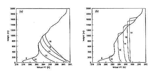
Fig.1. Profiles of from experiments D1 (a) and SC1 (b).

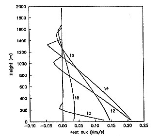
Fig.2. Profiles of vertical turbulent fluxes of from SC1.

Fig.1b shows a well-mixed boundary layer that deepens with time as the positive heat and moisture fluxes are applied at the surface through the initial 7 hours. A slight superadiabatic layer near the surface is evident, which agrees with observations. The scheme also produces overshooting at the top of the PBL, associated with which is entrainment of cold air at that level. The time evolution of these profiles is similar to observations (Clarke et al. 1971) and to previous simulations (e.g., André et al. 1978; Sun and Chang 1986).

The profiles of vertical fluxes are given in Fig.2 for SC1. The profiles are nearly linear with height and have distinct negative values near the PBL top that are about 15 to 20% of the surface values, again reflecting the presence of PBL top entrainment. It should be noted that the amount of entrainment is somewhat sensitive to the determination of the PBL top height (z_i) used in Eq.(1).

Now we turn to 3-D experiments. With x= 125 m and z=50m in D3A and SC3A, the 3-D runs can be referred to as large eddy simulations (LES). This setup is the same as that in Deardorff (1980). In these runs, 0.1 degree initial random perturbations were added at the lowest model level to the horizontally homogeneous potential temperature field so as to trigger convective eddies. The ensemble-averaged (averaged in horizontal and in time) profiles are shown in Fig.3 for D3A (a) and SC3A (b). In both cases, well-mixed profiles similar to those of SC1 are obtained, with the profiles in SC3A being slightly more vertical and the PBL slightly deeper than in D3A. Despite these similarities, the mechanisms by which the profiles were reached are somewhat different.

In D3A, the transport by parameterized (SGS) fluxes is very small except in the lowest 100 m. Above this layer, the resolved eddy transport accounts for most of the vertical mixing. The sum of the two parts, however, makes up nearly linear profiles of that are very close to those in SC1. In SC3A, the resolved eddy transport is weaker because part of the convective instability is removed by the strong vertical mixing associated with the PBL parameterization. Thus, less energy is left to feed convective eddies. This behavior is more prominent in runs with larger horizontal grid spacings (SC3B and SC3C, plots not shown) and suggests that the Sun and Chang type parameterization is suitable for cloudscale as well as mesoscale modeling as far as the ensemble-averaged effect of PBL turbulence is concerned. It will not be a good choice when detailed structures of eddies are of interest. The above results also suggest that when using the Sun and Chang type parameterization in a 3-D model with an eddy-resolving grid spacing, there does not seem to be a `double counting' effect, which answers the question we raised earlier in the Introduction.

We return again to the 3-D runs with Deardorff scheme. Fig.4 shows the profiles from D3C, in which x=6 km. The shape of the profiles appear very similar to those in the 1-D run (D1) until 16 h EST, when convective eddies are eventually induced by the strong convective instability accumulating during the previous hours. While sensitivity experiments show that the time of this onset depends on the initial perturbation size and the amount of numerical smoothing applied (we used a minimum smoothing just enough to suppress 2 x waves), the general behavior is true of all cases. This behavior was also observed in early stormscale simulations starting from 3-D analyzed data sets when neither a relatively crude flux-distribution procedure (see Xue et al. 1995) nor the current implementation of Sun and Chang was used.

After 16 h, instability that has been accumulating at the low-levels is released through the convective eddies. The resultant PBL is, however, too deep (about 2 km instead of the observed 1.3 km) and the stratification is stable rather than nearly neutral in the upper part of the PBL. The profiles of resolved and unresolved fluxes (not shown) are revealing; they show that the latter is responsible for most of the vertical heat transport before 16 h, whereas the former is small at all times except at 16 h, when the flux is positive and large below 800 m and negative and large above. Clearly, most of the convective instability was released at around 16 h in a less than one hour period and this impulsive release produced significant overshooting and excessive entrainment at the upper levels that are not very realistic (Fig.4). Similar behavior is observed in the 1 km resolution run with Deardorff scheme (D3B) although the results are closer to observations. This suggests that the 1 km resolution is still not sufficient to properly resolve even large convective eddies.

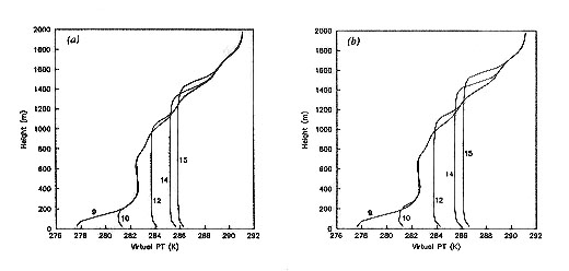
Fig.3. Plane-averaged profiles of from experiments D3A (a) and SC3A (b).

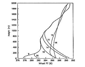
Fig.4. Plane-averaged profiles of from experiment D3C.

4. ACKNOWLEDGMENT

This research was supported by the Center for Analysis and Prediction of Storms at the University of Oklahoma, which is supported by NSF grant ATM91-20009 and a supplementary grant through NSF by Federal Aviation Administration. The authors benefited from comments by Dr. Vince Wong.

REFERENCES

André, J.C., et al., 1978: J. Atmos. Sci , 35, 1861-1883. Blackadar, A.K., 1979: Adv. Environ. Sci. and Eng., Vol.1, No.1, J. Pfafflin and E. Ziedler, Eds., Gordon and Breach, 50-85. Caughey, S. J. and S.G. Palmer, 1979: Q. J. Roy. Met. Soc., 105, 811-827. Clarke, R.H., et al., 1971: The Wangara experiment: Boundary layer data. Tech. Paper. 19, Div. Meteor. Phys. CSIRO, Australia. Deardorff, J. W., 1974a: Bound. Layer Meteor., 7, 81-106. _______, 1974b: Bound. Layer Meteor., 7, 199-226. _______, 1980: Bound. Layer Meteor., 18, 495-527. Klemp, J. B., and R. B. Wilhelmson, 1978: J. Atmos. Sci., 35, 1070-1096. Mellor, G. L., and T. Yamada, 1974: J. Atmos. Sci , 31, 1791-1806. _______, and T. Yamada, 1977: Proc. Symp. on Turbulenct Shear Flows. Penn. State Univer., 1-14. Sun, W.Y., and Y. Ogura, 1980: J. Atmos. Sci ., 37, 1558-1572. _______, and C-Z Chang, 1986 (SC86): J. Climate Appl. Meteor. 25, 1445-1453. Wyngaard, J.E., and O.R. Coté, 1974: Bound. Layer Meteor., 7, 289-308. Xue, M., et al. 1995: ARPS Version 4.0 User's Guide. 380pp. Available from the CAPS, U. of Oklahoma, Norman, OK, 73019. Zhang, D.-L., and R. A. Anthes, 1982: J. Appl. Meteor., 21, 1594-1609.