A Variational Method for the Analysis of Three-Dimensional
Wind Fields
from Two Doppler Radars
Jidong Gao*, Ming Xue*, Alan Shapiro*†
and Kelvin K. Droegemeier*†
*Center for Analysis and Prediction of Storms
†School of Meteorology
University of Oklahoma, Norman, Oklahoma 73019
(Revised manuscript for Mon. Wea. Rev., 21, August, 1998)
Downloard manuscript in PS format or Acrobat PDF format.
ABSTRACT
In this paper, we propose a new method of dual-Doppler radar analysis based on a variational approach. In it, a cost function, defined as the distance between the analysis and the observations at the data points, is minimized through a limited memory, quasi-Newton conjugate-gradient algorithm with mass continuity equation imposed as a weak constraint. The analysis is performed in Cartesian space.
Compared with traditional methods, the variational method offers much more flexibility in its use of observational data and various constraints. Using the radar data directly at observation locations avoids an interpolation step, which is often a source of error, especially in the presence of data voids. In addition, by using the mass continuity equation as a weak instead of strong constraint, we avoid the error accumulation and the subsequent somewhat arbitrary adjustment associated with the explicit vertical integration of the continuity equation.
The current method is tested on both model simulated and observed data sets of supercell storms. It is shown that the circulation inside and around the storms, including the strong updraft and associated downdraft, are well analyzed in both cases. Furthermore, we found that the analysis is not very sensitive to the specification of boundary conditions and to data contamination. The method also has the potential for retrieving, with reasonable accuracy, the wind in regions of single Doppler radar coverage.
1. Introduction
Doppler radar has long been a valuable observational tool in meteorology. It has the capability of observing, at high spatial and temporal resolution, the internal structure of storm systems from remote locations. However, the direct measurements are limited to reflectivity, the radial component of velocity, and the spectrum width: there is no direct measurement of the complete three-dimensional (3-D) wind field. In order to gain a more complete understanding of the atmosphere, it is desirable to know the full wind field.
When an atmospheric volume is observed simultaneously by two non-collocated Doppler radars, two degrees of freedom of 3-D wind vectors are determined. Techniques have been developed since the late 1960's to produce so-called dual-Doppler analyses. These techniques can be divided into two categories in term of the analysis geometry: 1) those in cylindrical coordinates, and 2) those in Cartesian space. Early dual-Doppler analyses stressed the synthesis of two independent Doppler velocity estimates in cylindrical coordinates (e.g., Armijo 1969; Lhermitte and Miller 1970; Miller and Strauch 1974). Doviak et al. (1976) performed a detailed error evaluation applicable to these dual-Doppler analyses. To improve vertical velocity estimates, Ziegler (1978) proposed a variational dual-Doppler analysis to deal with the problem of upper boundary condition.
Many other dual-Doppler synthesized analyses were performed directly in the Cartesian coordinate system. Brandes (1977) used a dual-Doppler analysis scheme in which wind components were synthesized from Doppler observations directly within a Cartesian grid, bypassing analysis procedures in cylindrical coordinates. Ray et al. (1980, 1981) designed a system to analyze data from multiple Doppler radars and tested it on a data set acquired by 2-4 radars during a field experiment over Oklahoma. It used a variational adjustment to improve vertical velocity estimates based on the mass continuity equation. Recently, Sun and Crook (1997, 1998) used adjoint approach to do the dual analyses and microphysical retrieval. They tested the method using both simulated data and real data, although this is an exciting development, but their computational requirements may currently prohibit their use in an operational setting. Compared to those methods solved in COPLAN coordinates (cylindrical space), the Cartesian methods require only one interpolation. Further, the grid may be aligned in the cardinal directions regardless of the orientation of the radar system.
The dual-Doppler analysis methods have greatly aided our understanding weather phenomena ranging from mesoscale convective complexes to clear air boundary layers . However, they still suffer from notable deficiencies, including the setting of vertical velocity boundary conditions, spatial interpolation errors, discretizations, uncertainties in radial wind estimates (due to sidelobes and ground clutter), and the non-simultaneous nature of the measurements. These problems have been discussed in Miller and Strauch (1974), Ray et al. (1975), Ray et al. (1980), Gal-chen (1982), Testud and Chong (1983), Chong and Testud (1983), Ziegler et al. (1983) and Shapiro and Mewes (1998).
The most pronounced difficulties concern the vertical velocity boundary condition and interpolation procedure. The natural boundaries for the problem are the irregular boundaries of the data region itself. If the region of dual-Doppler data coverage extends all the way to ground, then the impermeability condition could be safely applied. Unfortunately, the lower data boundary often lies hundreds to thousands of meters above ground level, where it is often inappropriate to apply the impermeability condition directly.
When the analysis is performed in a COPLAN coordinate system, it usually includes two steps: interpolation from a spherical coordinate system to a COPLAN coordinate system, and interpolation from a COPLAN coordinate system to a Cartesian coordinate system after the analysis is completed. Because of the irregular spatial distribution of the radar observations, large intervals between elevation angles (as large as 5 to 6 degrees for WSR-88D radar data), and the presence of bad data values, significant error can be introduced in the interpolation processes.
In the present paper, a new technique, based on a variational approach, permits flexible use of radar data in combination with other observations as well as the use of various constraints through the definition a cost function. In particular, by applying the anelastic mass conservation equation as a weak constraint, the severe error accumulation in the vertical velocity can be reduced because the explicit integration of anelastic continuity equation is avoided.
In addition, this method combines interpolation and analysis into a single step. The analysis is performed more naturally and directly in a Cartesian coordinate system, only interpolation from regular Cartesian grid to irregular radar observation points is needed. Since this interpolation process is usually well defined, the error should be smaller than when interpolation is done from a regular Cartesian coordinate system to an irregular radar coordinate system (Gao et al. 1995). Further, this reverse interpolation procedure preserves the radial nature of radar observations.
This paper is organized as follows: in Section 2, the variational method is introduced and a traditional dual-Doppler observation synthesis method is reviewed for reference. In Section 3, the variational method is tested on a set of idealized data sampled from a simulated supercell storm for which the true wind field is known. In section 4, we apply this variational method to a dual-Doppler data set from a tornadic supercell storm that occurred on 17 May 1981 near Arcadia, Oklahoma. Finally, summary and concluding remarks are given in Section 5.
2. Description of methodology
1) A variational dual Doppler analysis method
Variational analysis is a procedure that minimizes a cost function
J defined here to be the sum of squared errors due to the misfit between observations
and analyses subject to constraints. Each constraint is weighted by a factor
that accounts for its accuracy. There are different forms of ![]() that might be considered, and each one of them will give a different result
for the best-fit model solution. The variational method makes use of the derivative
of
that might be considered, and each one of them will give a different result
for the best-fit model solution. The variational method makes use of the derivative
of ![]() with respect to the analysis variables
and
with respect to the analysis variables
and ![]() must therefore be differentiable.
In our dual-Doppler radar analysis, we define the cost function as follows:
must therefore be differentiable.
In our dual-Doppler radar analysis, we define the cost function as follows:
(1)
(2)
(3)
(4)
(5)
Here ![]() is the difference
between the analyzed radial velocity
is the difference
between the analyzed radial velocity ![]() = (xu+yv+zw)/r and the observed radial velocity
= (xu+yv+zw)/r and the observed radial velocity ![]() ;
m is the number of radars; n is the number of observations; C
is a linear interpolation operator that maps
;
m is the number of radars; n is the number of observations; C
is a linear interpolation operator that maps ![]() from the grid (Cartesian coordinates) to observation points (spherical coordinates);
and u, v, and w are wind components in Cartesian coordinates
(x, y, z). It should be pointed out that the cost function can include
other observations that directly or indirectly measure u, v, and w. They include
soundings, single-level surface observations, aircraft data, or even satellite
observations.
from the grid (Cartesian coordinates) to observation points (spherical coordinates);
and u, v, and w are wind components in Cartesian coordinates
(x, y, z). It should be pointed out that the cost function can include
other observations that directly or indirectly measure u, v, and w. They include
soundings, single-level surface observations, aircraft data, or even satellite
observations.
![]() , the second term
of the cost function measures of how close the variational analysis is to the
background fields. The third term,
, the second term
of the cost function measures of how close the variational analysis is to the
background fields. The third term, ![]() ,
imposes a weak anelastic mass constraint on the analyzed wind field,
,
imposes a weak anelastic mass constraint on the analyzed wind field,
, (6)
where, ![]() is the mean
air density in the horizontal level.
is the mean
air density in the horizontal level.
The last term in the cost function, ![]() ,
is a smoothness constraint.
,
is a smoothness constraint.
Note that in the cost function, there exist several coefficients
such as ![]() and
and ![]() that are commonly referred to as penalty constants. Some of these coefficients
are matrices in general data assimilation methods. In storm-scale data assimilation,
especially with radar data, they are usually difficult to obtain.
that are commonly referred to as penalty constants. Some of these coefficients
are matrices in general data assimilation methods. In storm-scale data assimilation,
especially with radar data, they are usually difficult to obtain.
One of the major challenges of variational methods is the specification
of ![]() . For our purpose, these coefficients
are chosen according to the relative importance of each term. Experience with
the test cases presented herein suggests that the solutions obtained are not
very sensitive to the precise values of
. For our purpose, these coefficients
are chosen according to the relative importance of each term. Experience with
the test cases presented herein suggests that the solutions obtained are not
very sensitive to the precise values of ![]() ,
and therefore it is appropriate to treat the
,
and therefore it is appropriate to treat the ![]() as tuning parameters. Typically, the analysis changes by only a small amount
when a particular
as tuning parameters. Typically, the analysis changes by only a small amount
when a particular ![]() is halved or doubled,
but the minimizing analysis does change as expected for large changes in the
is halved or doubled,
but the minimizing analysis does change as expected for large changes in the
![]() (Hoffman 1984).
(Hoffman 1984).
To solve the above variational problem by direct minimization,
we need to derive the gradient of the cost function with respect to the control
variables (u, v, and w). Taking the variation with respect to
u, v and w, we obtain the components of the gradient of ![]() as
follows:
as
follows:
(7)
(8)
(9)
Here, C* is the adjoint of operator C. In the above, the commutation formula
(10)
of the finite-difference analog is used (Sasaki 1970), where we have specified values of u, v, w at the boundaries, that is,
(11)
(Note: in coding the program, the derivations above are performed
in its finite-difference analog. For clarity, we write them here in their continuous
form). It can be also noted that setting the gradients ![]() ,
,
![]() ,
, ![]() in
(7) - (9) to zero, yields three coupled Euler-Lagrange equations.
in
(7) - (9) to zero, yields three coupled Euler-Lagrange equations.
After the gradients of cost function are obtained, the problem can be solved in the following way:
(1) Choose the first guess of control variable Z=(u, v, w) (in our experiment, all first guesses are zero);
(2) Calculate the cost function according to Eqs. (1)-(5);
(3) Calculate the gradients ![]()
![]() and
and ![]() according to Eqs. (7)-(9);
according to Eqs. (7)-(9);
(4) Use a conjugate gradient method (Navon, 1987) to obtain update values of control variables,
![]() , (12)
, (12)
where, n is the number of iterations, ![]() is an optimal step size, obtained by the so-called "line search"
process in the optimal control theory (Gill et al 1981), and
is an optimal step size, obtained by the so-called "line search"
process in the optimal control theory (Gill et al 1981), and ![]() is the optimal descent direction obtained by combining the gradients from
several former iterations;
is the optimal descent direction obtained by combining the gradients from
several former iterations;
(5) Check if the optimal solution has been found by computing
the norm of the gradients or the value of ![]() to see if it is less than a prescribed tolerance. If the criterion is satisfied,
stop iterating and output the optimal u, v and w;
to see if it is less than a prescribed tolerance. If the criterion is satisfied,
stop iterating and output the optimal u, v and w;
(6) If the convergence criterion is not satisfied, steps 2 through 5 are repeated using updated values of u, v, and w as the new guess. The iteration process is continued until a satisfactory solution is found.
2) Conventional synthesis method
To highlight the differences between traditional dual-Doppler analysis approaches and our variational analysis method, the procedure of a traditional method is briefly reviewed here. It follows closely the widely-used dual-Doppler analysis technique contained in the NCAR software package CEDRIC (Mohr 1988).
The radial velocity Vr at a point (X, Y, Z) can be expressed as
(13)
where,
(14)
u, v, and w are the Cartesian velocity components (Mohr, 1988). This notation is used to conform to that for traditional ground-based dual-Doppler analysis.
For two radars, we let P be A and B, respectively, and we obtain the following formula from (13) and (14):
(15)
(16)
where D= XA YB - XB
YA, ![]() =(YAZB
- YBZA)/D, and
=(YAZB
- YBZA)/D, and ![]() =(XBZA
- XAZB)/D. With data from only two radars, u,
v and w are not explicitly determined, But for a good "first guess",
the w terms can be neglected, yielding the following estimates for the horizontal
velocities:
=(XBZA
- XAZB)/D. With data from only two radars, u,
v and w are not explicitly determined, But for a good "first guess",
the w terms can be neglected, yielding the following estimates for the horizontal
velocities:
, (17)
, (18)
The factors![]() and
and![]() become
geometric multipliers that can be used to adjust the estimates u' and
v' if w is found using other information.
become
geometric multipliers that can be used to adjust the estimates u' and
v' if w is found using other information.
The vertical velocity estimate is usually obtained by integrating the anelastic mass continuity equation (6) upward (or downward) subject to the boundary condition w = 0 at the lower boundary (or upper boundary). An O’Brien wind adjustments (O'Brien 1970) is typically applied to ensure that w = 0 at both boundaries. The horizontal velocity components are then recomputed as
, (19)
. (20)
With this simple approach, the velocities are calculated and corrected by an iterative procedure. First, an approximate w is obtained by integrating the continuity equation (based on the approximate horizontal velocities). The horizontal velocities are then corrected, and the process is repeated until a convergence criterion is met.
3) The effect of terminal velocity
With both variational and traditional methods, the fall speed of precipitation has to be taken into account. For radar scans at a non-zero elevation angle, the fall speed of precipitation particles contributes to the Doppler estimate of radial velocity. The observations of radial velocity are adjusted to remove this contribution, using (Foote and duToit 1969; Atlas et al. 1973)
. (21a)
where ![]() is the air
radial velocity,
is the air
radial velocity, ![]() is the target radial velocity, wt is the terminal velocity
of precipitation, and
is the target radial velocity, wt is the terminal velocity
of precipitation, and ![]() is the elevation
angle (00 is horizontal).
is the elevation
angle (00 is horizontal).
The adjustment to radial velocity in Eq. (21a) is based on an empirical relationship between reflectivity factor and raindrop terminal fall velocity (Atlas et al. 1973):
. (21b)
Here Z is the reflectivity, ![]() the air density, and
the air density, and ![]() the air density
at the surface.
the air density
at the surface.
3. Tests with simulated data
1) Experimental design
To evaluate the performance of our variational analysis method and compare it with the more traditional method outlined in the previous section, we utilize a set of simulated dua-Doppler data. This strategy is often called OSSE (Observation System Simulation Experiments) experiments. A well-documented tornadic supercell storm that occurred near Delcity, Oklahoma on 20 May 1977 is used for the numerical experiments. This storm has been studied extensively, using both multiple Doppler analysis and numerical simulation. For details on its morphology and evolution, readers are referred to Ray et al. (1981), Klemp et al. , and Klemp and Rotunno (1983).
The Advanced Regional Prediction System (ARPS, Xue et al. 1995) is used here to perform a two-hour simulation of this storm. The simulation starts from a thermal bubble placed in a horizontally homogeneous base state specified from the sounding used in Klemp et al. (1981). As in Klemp et al. (1981), a mean storm speed (U=3 ms-1, V=14 ms-1) is subtracted from the sounding to keep the right-moving storm near the center of model domain.
The model grid is comprised of 67x67x35 grid points and the grid interval is 1 km in the horizontal and 0.5 km in the vertical. The physical domain size is 64x64x16 km3. The storm is initiated by an isolated thermal bubble centered at x = 48 km, y = 16 km and z = 1.5 km, with the origin at the lower left corner of the grid. The radius of the bubble is 10 km in both x and y directions and 1.5 km in the vertical direction. The magnitude of the thermal perturbation is 4 degrees. Kessler (1969) warm rain microphysics is used together with a 1.5-order turbulent kinetic energy sub-grid parameterization. Open boundary conditions are used at the lateral boundaries while an upper-level Rayleigh damping layer is included to reduce wave reflection from the top of the model.
By two hours into the simulation, the initial storm has undergone a splitting process , with the right-mover remaining near the center of the domain and the left mover propagating to the northwest corner. Figure 1 shows horizontal and vertical cross-sections of wind, vertical velocity (vertical section is plotted through line A-B in Fig.1a), and reflectivity fields at two hours. A strong rotating updraft (with maximum vertical velocity exceeding 34 m/s) and associated low-level downdraft are evident near the center of the domain while disturbances associated with the left mover are also clear. Downstream of the over-shooting updraft at the tropopause level are downward returning flows that exhibit gravitational oscillations (Fig.1b). The evolution of the simulated storm is qualitatively similar to that described by Klemp and Wilhelmson , and by two hours, has attained a structure typically of mature supercell storms.
The simulated 3-D convective-scale wind field at two hours is sampled by two pseudo-radars, the locations of which relative to the grid are shown in Fig. 2. The wind components are first interpolated using a Cressman scheme (1959) from the model grid points to the sampling locations along the radar beams with the influence radius R = 2.5 km, and are synthesized to obtain radial velocities according to Eq. (13). The elapsed times for the volume scans of two radars are neglected, and thus we presume that the radial wind observations are simultaneous.
Radar A in Fig. 2 covers a horizontal
area of 10 km < r < 80 km and ![]()
![]() <
< ![]() <
< ![]() ,
where r is the radius and a
is the azimuthal angle. Radar B covers a horizontal area
of 10 km < r < 80 km and
,
where r is the radius and a
is the azimuthal angle. Radar B covers a horizontal area
of 10 km < r < 80 km and ![]() <
< ![]() <
< ![]() .
The gate spacing is 500 m, the azimuthal angle is
.
The gate spacing is 500 m, the azimuthal angle is ![]() ,
and the elevation angle is
,
and the elevation angle is![]() . The lowest
elevation angle is
. The lowest
elevation angle is ![]() . The simulated
data is only specified in precipitation regions (where reflectivity is greater
than zero) covered by both radars. In order to simulate the radar’s statistical
error, random errors with different magnitudes are added to the radial velocities
in three of the experiments.
. The simulated
data is only specified in precipitation regions (where reflectivity is greater
than zero) covered by both radars. In order to simulate the radar’s statistical
error, random errors with different magnitudes are added to the radial velocities
in three of the experiments.
To measure the accuracy of the dual-Doppler analysis, we calculate the following error statistics.
The RMS error and relative RMS error of the horizontal winds are given by:
RMSV =
, (22)
RREV =, (23)
And the RMS error and relative RMS error of the vertical velocities are likewise given by:
RMSW =
, (24)
RREW =. (25)
Here N represents the total number of grid points for u, v, and w in the area covered by the two Doppler radars. The subscript ref stands for the reference or actual field from the ARPS model solution. In addition, the correlation coefficients (CC) of horizontal and vertical wind between the retrieved field (u, v, and w) and reference fields (uref, vref, and wref) are also calculated for each experiment.
2) Results of analysis
In this section, we present the results from a set of OSSE's experiments outlined in the previous section. The analysis domain is the same as the ARPS integration domain described earlier, and the experiments are listed in Table 1. Among them is the control run (CNTL), the results of which are shown at three minimization iteration steps 50, 100, and 200. Two more experiments are performed to examine the effect of a weak mass continuity constraint (NOMC) and spatial smoothing (NOSM). The perfect OSSE data are used for these experiments. Finally, experiments ERR1 through ERR3 test the error tolerance of the variational method by adding some errors to the OSSE data. The first guesses for all of the experiments are zero. The horizontally homogeneous background field is specified from a single sounding of May 20, 1997 at Del City, Oklahoma.
The parameter settings used are ![]() ,
,
![]() ,
, ![]() ,
,
![]() , and
, and ![]() =
0.5x10⁻³. These values are chosen so that the constraints are of
roughly the same order of magnitude after being multiplied by the coefficients.
These parameters also indicate the relative importance of each term in the cost
function.
=
0.5x10⁻³. These values are chosen so that the constraints are of
roughly the same order of magnitude after being multiplied by the coefficients.
These parameters also indicate the relative importance of each term in the cost
function.
We first examine the number of iterations needed to minimize J. Generally speaking, the optimal number is case-dependent, and is also a function of the pre-conditioning and minimization method used. In practice, the appropriate number of iterations can be estimated by examining the behavior of cost function, i.e., the minimization process can be stopped when the change in the cost function becomes small. Fig. 3 shows that the cost function starts to level off after 100 iterations in the control experiment. From about 150 to 300 iterations, the curve of cost function becomes essentially horizontal, although the norm of gradient still decreases further.
The quality of the retrieval can be ascertained by the RMS errors and correlation coefficients, and by comparing the retrieved fields with the "exact" solution from the ARPS model. The error statistics for various numbers of iterations are shown in Table 1. The RMS errors and correlation coefficients for the horizontal wind change very little after 50 iterations; however, the vertical velocity retrieval continues to improve thereafter.
To examine the quality of the analysis more closely, we show in Figs. 4-5 sample plots for iteration steps 50 and 200 respectively. Comparing with the true fields in Fig. 1, all the features in the horizontal winds, i.e., the curvature around the rotating updraft and the convergence, are well retrieved. However, the flow in the vertical cross-section is significantly different in Figs. 4b-5b. Although the general structure of updraft is retrieved after only 50 iterations, the maximum vertical velocity is very low (21.62 m/s) compared to the "true" one (43.55m/s). At middle and upper levels, the downdraft in the eastern part of model domain is not present. Oscillations downstream of the updraft top due to gravitational waves are also missing. For iteration 100 (not shown), the maximum updraft is still low (30.12 m/s) and the downdraft at mid levels is retrieved. However, the downdraft at the upper levels is still missing. At 200 iterations, both the horizontal and vertical winds are well recovered (see Fig. 5). The analyzed 3D wind fields are reasonably close to the true wind fields in Fig. 1. The relative RMS errors at this iteration step are less than that of the other two steps in Table 1. Thus, in the minimization process, the number of iterations needed to obtain a good retrieval is very different for the horizontal and vertical winds.
To obtain the reasonable horizontal wind analysis, only a small number of iterations are needed. This is, because Doppler radars usually operate at low elevation angles, the horizontal winds are well observed. The absolute values of the gradient of the cost function with respect to horizontal winds for the first iteration are relatively large when compared to those for the vertical velocity (not shown). Hence, the cost function is more sensitive to horizontal winds than vertical winds, and therefore the horizontal wind component is easily retrieved with sufficient accuracy in only 50 iterations. The contribution of vertical velocity to the observed radial velocities is, however, relatively small due to the small elevation angles, and thus the analysis still contains large errors after first 50 iterations. After that, the absolute values of the gradient of the cost function with respect to horizontal and vertical winds become the same order of magnitude and the mass continuity constraint becomes effective. The vertical velocity becomes well retrieved after 200 iterations because of adjustments to this constraint giving better-retrieved horizontal winds. From iterations 200 to 300, the accuracy of both the horizontal and vertical wind remains essentially unchanged and thus we terminate the analysis after 200 iterations.
3) The role of the anelastic mass continuity constraint
Our variational analyses show satisfactory results of 3-D dual-Doppler wind analysis, including the vertical velocity. To explain the role of the weak mass continuity constraint, we perform experiment NOWC (see Table 1) which is exactly the same as the control (CNTL) case except that the mass continuity constraint is removed.
As shown in Table 1, both the RMS error and correlation coefficients indicate that the horizontal wind are recovered with reasonable accuracy; however, the retrieval of vertical velocity is poor. Figure 6b shows that no coherent structure in w is retrieved below 4km, but results above 4km are qualitatively good. This is not surprising, though, because very limited information on w is contained in the radial wind observations at low levels.
With conventional methods, the vertical velocity is obtained by integrating the mass continuity equation, and in this sense, the equation is used as a "strong constraint". The main difficulty lies in specifying the w boundary conditions. The requirement of zero vertical velocity at the ground is the most natural physical condition (Miller and Strauch 1974; Doviak et al. 1976). However, it was later demonstrated that upward integration of vertical velocity was unreliable because the bias errors in the divergence field can be amplified exponentially with height (Ray et al. 1980).
To reduce the accumulation of w error, Ziegler (1978) proposed a dual-Doppler analysis that incorporated boundary conditions w = 0 at z = 0 and w = - vt at the upper data boundary (vt terminal velocity, which was small in his study). Further, Ray et al. (1980) applied a variational wind adjustment to the analyzed winds in their multiple Doppler radar analysis. The anelastic mass continuity equation was used as a strong constraint in both cases.
The vertical integration of the anelastic mass continuity equation is particularly difficult for our simulated data set because of the presence of large data void areas. For example, the lower boundary of the radar echo is as high as 6 km in certain vertical columns (see Fig.1b). The resultant w field from such integration can be very problematic even if an additional variational adjustment is applied. It is therefore advantageous to apply the mass continuity equation as a weak constraint so that explicit integration of the equation is avoided. By doing so, to specify w boundary conditions explicitly at data boundary is not needed. However, the use of the background field and/or the smoothness constraint still permits us to set w equal zero at both model top and bottom.
To summarize, in conventional dual-Doppler techniques, the horizontal and vertical winds are derived in two separate steps. With our method, the horizontal and vertical wind components are retrieved together, subject to the weak constraint of anelastic mass continuity. The use of a weak instead of strong constraint also leads to procedural simplicity in that the explicit solution of an elliptic equation that would arise from the use of a strong constraint is avoided. The latter tends to be sensitive to the specification of boundary conditions. This finding also agreed with Xu and Qiu's (1994) when they compared the advantages and disadvantages of using weak versus strong constraint of mass continuity in the so-called simple adjoint techniques.
4) The role of smoothing
In addition to the physical constraints, a smoothness constraint, Js, as proposed by Thacker (1988), is added to the cost function J. Yang and Xu (1996) discussed theoretically the role and effect of spatial smoothness constraint on statistical errors in variational data assimilation in their simple one-dimensional model. Sun and Crook (1994) found the accuracy of retrieval results can be greatly improved when smoothness constraint was used in their experiments. Table 1 shows that, when this smoothness term is excluded from the cost function (experiment NOSM), the retrieval results deteriorate, especially for the vertical velocity. The analyzed 3D wind fields (Fig. 7) lack of coherence and contain significant noises. From this test, the importance of smoothness is clear: The inclusion of the smoothness term improves the 3D-wind analysis by removing small-scale noises, and also helps to increase the area of influence of the radar data. The latter is more important in the vertical direction since the separation between observations is often large; for WSR-88D data, the scans can be more than several degrees apart in elevation angle.
From Tables 1, it can be seen that the relative impact of smoothing versus anelastic mass continuity equation on the horizontal wind field is about the same, but mass continuity is much more important than smoothing for vertical velocity. Lack of smoothing alone increases RMS error for vertical velocity by about 0.7 m/s over the control run; but lack of mass continuity alone increases RMS error for vertical velocity by about 3.3 m/s.
5) Relaxation to the background
When radar data are to be used to initialize a numerical weather prediction (NWP) model, a complete description of the wind and other meteorological variables is needed in the entire model domain. Even for diagnostic studies, consistent analysis outside the radar data areas is also desirable. Conventional observations such as the rawinsondes, or background fields from NWP models, can be used to complement the radar data. However, there is the issue of blending the radar data with the background information.
Lin and Ray (1993) proposed a method for obtaining a smooth transition from regions with radar observations to the ambient environment defined by a single sounding. Using the analyzed u and v fields at the data boundaries as the "inner" Dirichlet boundary condition and a single rawinsonde as the "outer" Dirichlet boundary condition (i.e., on the domain boundary), they solved two Laplace equations for u and v which minimize the horizontal gradients of u and v in the data-void areas. Because the u and v fields so obtained do not satisfy mass continuity in general, they applied an additional mass-continuity variational adjustment. Nevertheless, on the boundary between the original radar data and the filled data, the space derivatives of the wind field were discontinuous (Lin and Ray 1993).
Ellis (1997) also used OSSE to study hole-filling the data voids in simulated radar data. Two different hole-filling techniques were involved in his method: The first one was similar to that of Lin and Ray (1993); the second one minimized the second derivative of the scalar field being filled. In both cases the variational wind adjustment of Ray et. al (1981) was then applied to the hole-filled wind field. He found the first technique performed generally better than the second one. The variational wind adjustment improves the statistics of each hole-filling wind field.
With the variational method proposed here, the several
steps commonly used in conventional methods are effectively combined into a
single step. The rawinsonde (and other available) data are incorporated into
the cost function to automatically fill the data-void regions. The weighting
constant for the background field should be properly selected, and should be
large enough to keep the wind outside the precipitation regions close to the
background, but not too large so as to lessen the fit of the analysis to radar
observations. In our experiments, we find that ![]() ,
,
![]() works well.
works well.
To examine the effectiveness of using a single sounding to specifying the background environment, we repeat the control experiment without the background sounding. The analyzed winds are plotted for the entire domain in Fig. 8 and compared with those of control case, re-plotted for the same domain in Fig.9. In the analysis without a background, no information is available outside the data areas, the analysis remains largely unchanged from the first guess, which in our case is zero (Fig 8). However, for the control case, though no observational constraint is available outside the radar-observed data areas, the analysis takes on the values of the background and the transition is smooth between the data area and non-data area (Fig. 9). It is worth pointing out, that even though the analysis outside the radar data areas is very poor with strong horizontal convergence and divergence near the data boundaries, the analysis within the data coverage area is very good (c.f. Fig.8 and Fig.9). This again suggests that the current variational analysis is not very sensitive to data boundaries and parameters specified outside the radar-observed storm region.
It is also interesting to note that near the northwest corner of the domain, the left-moving storm is partially covered by a single radar (Radar B in Fig.2). Our analysis procedure is still able to retrieve some of the flow structure of this storm cell. This is possible due to the fact that with variational methods, one can make use of whatever information is available, and often in an optimal way; with traditional methods, whereas, dual-Doppler radar coverage is essential.
6) Sensitivity to random observational errors
In the above experiments, we have assumed
that the radial velocity observations are free of error. In reality, radial
velocity observation can contain large errors, especially some biased errors
(ground cluster, AP, etc.). However, it is very difficult to account for simulated
biased errors. In this section, we test the quality of the variational-analyzed
fields subject to random observational errors. Experiments ERR1, ERR2 and ERR3
(Table 1) involve the addition of 20, 60 or 100 % random errors, respectively,
to the radial velocity observations from both radars. In another word, we use
![]() as the observations, where e
represents random numbers between -1 and +1 and a
is 0.2, 0.6 and 1, respectively. When a = 0.2,
the relative RMS error for the horizontal wind is not significantly changed
from that of the control experiment (28 % versus 20.9 % for CNTL). However,
the relative RMS error of vertical velocity increases from 60.9 % to 80.8 %,
and the correlation coefficient decreases from 0.825 to 0.729. Thus, the vertical
velocity is more sensitive to observational errors than the horizontal wind.
Nevertheless, the general features of the 3-D wind field are well retrieved
(Fig. 10).
as the observations, where e
represents random numbers between -1 and +1 and a
is 0.2, 0.6 and 1, respectively. When a = 0.2,
the relative RMS error for the horizontal wind is not significantly changed
from that of the control experiment (28 % versus 20.9 % for CNTL). However,
the relative RMS error of vertical velocity increases from 60.9 % to 80.8 %,
and the correlation coefficient decreases from 0.825 to 0.729. Thus, the vertical
velocity is more sensitive to observational errors than the horizontal wind.
Nevertheless, the general features of the 3-D wind field are well retrieved
(Fig. 10).
When a is increased to 0.6, the retrieval of horizontal winds remains good, but the retrieved vertical velocity exhibits larger noise (figures not shown). In experiment ERR3, we give an extreme example by setting a to 1.0. This example shows that the method is rather robust even for such large observation errors. The relative RMS error of the horizontal winds remains reasonably small (0.43) and the correlation coefficient is as high as 0.91 (Table 1). However, the relative errors of the vertical velocity are as large as 1.24.
Fig. 11 shows considerable noise in both the horizontal and vertical wind fields. In spite of that, the general pattern of the flow is still rather similar to the pseudo observations.
4. Application to real data
In the previous section, we discussed results from a set of OSSE experiments using model-generated pseudo observations. To demonstrate the effectiveness of the variational method for real data, we apply our method to the 17 May 1981 Arcadia, OK supercell storm. Twelve coordinated dual-Doppler scans were obtained from the Norman and Cimarron, OK S-band Doppler radars over a one hour period spanning the pre-tornadic phase of the storm. Using the dual-Doppler analysis technique contained in the NCAR software package CEDRIC (Mohr 1988), Dowell and Bluestein (1997) performed a detailed dual-Doppler analysis of this storm which will serve as our benchmark. Due to the lack of third radar, neither our nor Dowell and Bluestein's analysis can be validated against a more accurate analysis, therefore the discussion will remain qualitative.
The results of our analysis for 1634 CST on 17 May are shown in Fig.12. At low levels (Fig.12a), a cold outflow is seen to originate from rear flank downdrafts that exhibit two maximum centers flanking the occlusion point of the gust fronts. Ahead of this outflow is the rear flank gust front which is associated with surface convergence and vertical velocity maximum. The reflectivity field shows a hook-echo pattern that is consistent with the retrieved flow. Such a flow structure is typical of a tornadic supercell storm with strong low-level rotation .
At mid-levels, a strong updraft core (>25 m/s) is retrieved that is roughly collocated with the mesocyclone (center of strong rotation) and reflectivity maximum (Fig.12b). In a vertical cross-section plotted through the line A-B in Fig.12a, the main updraft is seen to originate ahead of the low-level gust front. It reaches a maximum intensity of 35.42 m/s at the 8 km level and in general matches the areas of maximum reflectivity. The main downdraft is located below the updraft core and is collocated with a region of high reflectivity behind the gust front. These features suggest that both the horizontal and vertical flows are kinematically consistent. They also qualitatively agree with those analyzed in Dowell and Bluestein (1997).
5. Summary and concluding remarks
In this paper, we proposed and tested a variational analysis scheme that is capable of retrieving three-dimensional winds from dual-Doppler observations of convective storms. It was shown that the variational method has notable advantages over traditional dual-Doppler analysis techniques. The need for explicitly integrating the mass continuity equations and solving elliptic equations in the variational adjustment step, as well as the ‘hole-filling’ procedure, makes the analysis from traditional methods more susceptible to boundary condition uncertainties than the variational method here. In addition, separate interpolation from radar observation to analysis grid in traditional method is often source of errors.
The main conclusions can be drawn as follows:
It is our plan to generalize our variational analysis procedure to include additional data sources, and to introduce dynamic constraints in the cost function so that thermodynamical fields are retrieved simultaneously with the winds. This procedure is expected to further improve the wind analysis at the same time.
Acknowledgments This research was supported by NSF Grant ATM91-20009 to the Center for Analysis and Prediction of Storms (CAPS), by U.S. Department of Defense (Navy) Grant N00014-96-1-112 to A. Shapiro through the Coastal Meteorological Research Program (CMRP). The first author appreciates the enlightening discussions with Dr. Qin Xu at Navy Research Laboratory. Special thanks go to Steve Weygandt for providing the Arcadia storm data set, which came from Howard Bluestein and David Dowell. Graphics plots were generated by ZXPLOT graphics package written by Ming Xue. Computations were performed on the Pittsburgh Supercomputing Center Cray C90. Finally we would like to thank three anonymous reviewers for their very helpful comments which substantially improved the quality of this manuscript.
Reference
Armijo, L., 1969: A theory for the determination of wind and precipitation velocities with Doppler radars. J. Atmos. Sci., 26, 570-573.
Atkins, N. T., T. M. Weckwerth, and R. M. Wakimoto, 1995: Observations of the sea-breeze front during CaPE. Part II: Dual Doppler and aircraft analysis. Mon. Wea. Rev., 123, 944-969.
Atlas, D., R. C. Srivastava, and R. S. Sekhon, 1973: Doppler radar characteristics of precipitation at vertical incidence. Rev. Geophys. Space Phys., 11, 1-35
Brandes, E. A., 1977: Flow in severe thunderstorms observed by dual-Doppler radar. Mon. Wea. Rev., 105, 113-120.
Carbone, R. E., 1983: A severe frontal rainband. Part II: Tornado parent vortex circulation. J. Atmos. Sci., 40, 2639-2654.
Chong, M., J. Testud, and F. Roux, 1983: Three-dimensional wind field analysis from dual-Doppler radar data. Part II: Minimizing the error due to temporal variation. J. Climate Appl. Meter., 22, 1216-1226.
___, ___, and ___, 1983: Three-dimensional wind field analysis from dual-Doppler radar data. Part III: Minimizing the error due to temporal variation. J. Climate Appl. Meter., 22, 1227-1241.
Cressman, G. W., 1959: An operational objective analysis system. Mon. Wea. Rev., 87, 367-374.
Doviak, R. J., P. S. Ray, R. G. Strauch and L. J. Miller, 1976: Error estimation in wind fields derived from dual-Doppler radar measurement. J. Appl. Meteor., 8, 249-253.
Dowell, D. C., and H. B. Bluestein, 1997: The Arcadia, Oklahoma, storm of 17 May 1981: Analysis of a supercell during tornadogensis. Mon. Wea. Rev., 125, 2562-2582.
Ellis, S., 1997: Hole-filling data voids in meteorological fields. Master’s thesis, University of Oklahoma, 198pp.
Foote, G. B., and P. S. duToit, 1969: Terminal velocity of raindrops aloft. J. Appl. Meteor., 8, 249-253.
Gal-Chen, T., 1982: Errors in fixed and moving frame of references: Applications for conventional and Doppler radar analysis. J. Atmos. Sci., 39, 2279-2300.
Gao J., J. Chou, and L. Zhi, 1995a: A method for determining the spatial structure of meteorological variable from the temporal evolution of observational data. Chinese J. Atmos. Sci., 19, 113-125.
Gill, P. E., and W. Murray, and M. H. Wright, 1981: Practical Optimization. Academic Press, 401 pp.
Hoffman, R. N. 1984: SASS wind ambiguity removal by direct minimization. Part II: Use of smoothness and dynamical constraints. Mon. Wea. Rev. 112 1829-1852.
Kessinger, C., J., P. S. Ray, and C. E. Hane, 1987: The Oklahoma squall line of 19 May 1977. Part I: A multiple Doppler analysis of convective and stratiform structure. J. Atmos. Sci., 44, 2840-2864.
Kessler, E., 1969: On the distribution and continuity of water substance in atmospheric circulation. Meteor. Monogr., 10, No., 32, Amer. Meteor. Soc.
Klemp, J. B., and R. B. Wilhelmson, 1978: Simulations of right- and left-moving storms produced through storm splitting. J. Atmos. Sci., 35, 1097-1110.
Klemp, J. B., and R. B. Wilhelmson and P. S. Ray, 1981: Observed and numerically simulated structure of a mature supercell thunderstorm. J. Atmos. Sci., 38, 1558-1580.
Klemp, J. B., and R. Rotunno, 1983: A study of the tornadic region within a supercell thunderstorm. J. Atmos. Sci., 40, 359-377.
Lemon, L. R., and I. C. A. Doswell, 1979: Severe thunderstorm evolution and mesocyclone structure as related to tornadogenesis. Mon. Wea. Rev., 107, 1184-1197.
Lhermitte, R. M., and L. J. Miller, 1970: Doppler radar methodology for the observation of convective storms. Preprints, 14th Radar Meteor. Conf., Amer. Meteor. Soc., Tucson, Ariz., 133-138.
Lin, Y., P. S. Ray, and K. W. Johnson, 1993: Initialization of a modeled convective storm using Doppler radar-derived fields. Mon. Wea. Rev., 121, 2757-2775.
Miller, L. J., and R. G. Strauch, 1974: A dual Doppler radar method for the determination of wind velocities within precipitating weather systems. Remote Sens. Environ., 3, 219-235.
Mohr, C. G., 1988: CEDRIC - Cartesian Space Data Processor. NCAR, Boulder, Colorado, 78pp.
Navon, I. M., and D. M. Legler, 1987: Conjugate-gradient methods for large-scale minimization in meteorology. Mon. Wea. Rev., 115, 1479-1502.
O’Brien, J., J., 1970: Alternative solutions to the classic vertical velocity problem. J. Appl. Meteorol. 9, 197-203.
Parsons, D. B., and R. A. Kropfli, 1990: Dynamics and fine structure of a microburst. J. Atmos. .Sci., 47, 1674-1692.
Ray. P. S., R. J. Doviak, G. B. Walker, D. Sirmans, J. Carter and B. Bumgarner, 1975: Dual-Doppler observations of a tornadic storm. J. Appl. Meteorol. 14, 1421-1530.
___, C. L. Ziegler, W. Bumgarner, and R. J. Serafin, 1980: Single- and Multiple-Doppler radar observations of tornadic storms. Mon. Wea. Rev., 108, 1607-1625.
___, B. C. Johnson, K. W. Johnson, J. S. Bradberry, J. J. Stephens, K. K. Wagner, R. B. Wilhelmson, and J. B. Klemp, 1981: The morphology of several tornadic storms on 20 May, 1977. J. Atmos. Sci., 38, 1643-1663.
Reinking, R. F., R. J. Doviak, and R. O. Gilmer, 1981: Clear-air roll vortices and turbulent motions as detected with an air-borne gust probe and dual-Doppler radar. J. Appl. Meteor., 20, 678-685.
Sasaki, Y., 1970: Some basic formalisms in numerical variational analysis. Mon. Wea. Rev., 98, 875-883.
Shapiro A., and J. J. Mewes, 1998: New formulations of dual-Doppler wind radar. J. Atmos. Oceanic Technol. (in review).
Sun, J., and N. A. Crook, 1994: Wind and thermodynamic retrieval from single-Doppler measurements of a gust front observed during Phoenix II. Mon. Wea. Rev., 122, 1075-1091.
Sun, J., and N. A. Crook, 1997: Dynamical and microphysical retrieval from Doppler radar observations using a cloud model and its adjoint. Part I: Model development and simulated data experiments. J. Atmos. Sci., 54, 1642-1661.
Sun, J., and N. A. Crook, 1998: Dynamical and microphysical retrieval from Doppler radar observations using a cloud model and its adjoint. Part II: Retrieval experiments of an observed Florida convective storm. J. Atmos. Sci., 54, 1642-1661.
Testud, J. D., and M. Chong, 1983: Three-dimensional wind field analysis from dual-Doppler radar data. Part I: Filtering, interpolation and differentiating the raw data. J. Climate Appl. Meteor. 22, 1204-1215.
Thacker, W. C., 1988: Fitting models to inadequate data by enforcing spatial and temporal smoothness. J. Geopgys. Res, 93, 10655-10665.
Xu, Q., and C. J. Qiu, 1994: Simple adjoint methods for single-Doppler wind analysis with a strong constraint of mass conservation. J. Atmos. And Oceanic. Technol., 11, 289-298.
Xue, M., K. K. Droegemeier, Vince Wong, A. Shapiro, and K. Brewster, 1995: Advanced Regional Prediction System (ARPS) Version 4.0 User's Guide, 380 pp. [Available from Center for Analysis and Prediction of Storms, University of Oklahoma, 100E. Boyd, Norman, OK 73019].
Yang, S. and Q. Xu, 1996: Statistical errors in variational data assimilation -- A theoretical one-dimensional analysis applied to Doppler wind retrieval. J. Atmos. Sci. 53, 2563-2577.
Ziegler, C. L., 1978: A dual Doppler variational objective analysis as applied to studies of convective storms. Master’s thesis, University of Oklahoma, 116pp.
Ziegler, C., P. S. Ray, and N. C. Knight, 1983: Hail growth in an Oklahoma multi-cell storm. J. Atmos. Sci., 40, 1768-1791.
Table 1. List of experiments with simulated data set
|
Experiments |
Scheme |
Number of Iterations |
Horizontal wind(VH) |
Vertical wind (w) |
||||
|
RMS |
RRE |
CC |
RMS |
RRE |
CC |
|||
|
CNTL1 |
Control |
50 |
4.893 |
0.257 |
0.968 |
2.626 |
0.786 |
0.657 |
|
CNTL2 |
Control |
100 |
4.002 |
0.210 |
0.978 |
2.140 |
0.641 |
0.775 |
|
CNTL |
Control |
200 |
3.958 |
0.209 |
0.978 |
1.937 |
0.609 |
0.825 |
|
NOWC |
No weak- constraint |
200 |
4.019 |
0.211 |
0.978 |
4.225 |
1.265 |
0.222 |
|
NOSM |
No smoothness |
200 |
4.557 |
0.240 |
0.971 |
2.631 |
0.788 |
0.712 |
|
ERR1 |
20% errors |
200 |
5.356 |
0.282 |
0.960 |
2.572 |
0.808 |
0.729 |
|
ERR2 |
60% errors |
200 |
5.572 |
0.306 |
0.954 |
2.757 |
0.825 |
0.707 |
|
ERR3 |
100% errors |
200 |
8.237 |
0.434 |
0.910 |
3.948 |
1.241 |
0.544 |
|
ARCADIA |
Variational |
200 |
N.A. |
|||||
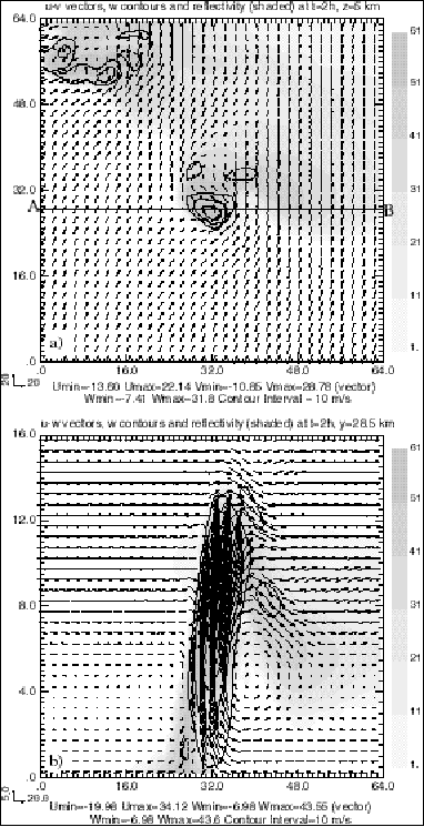
Figure 1. The ARPS model simulated wind vectors, vertical velocity w (contours) and simulated reflectivity (shaded) fields of the 20 May 1977 supercell storm at 2 hours. a) Horizontal cross-section at z = 5 km; b) Vertical cross-section at y=28.5 km, i.e., through line A-B in a).

Figure 2. Locations of the two assumed radars that sample data from the ARPS two hours run in Fig.1.
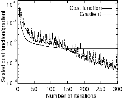
Figure 3. The scaled cost function (Jk/J0)
and scaled gradient norm (![]() ) as
a function of the number of iterations.
) as
a function of the number of iterations.
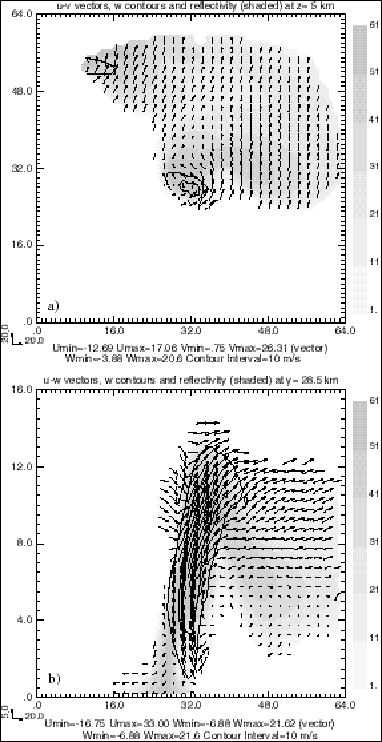
Figure 4. Wind vectors, vertical velocity (contours) retrieved from data sampled by two Doppler radars (see Fig.2) using the variational analysis method at iteration number 50. The horizontal cross-section is at z = 5km and vertical cross-section at y = 28.5, as shown in Fig.1 as line A-B. Also shown as shaded contours are the simulated reflectivity fields. Only analysis in the 'rainy' areas (areas with reflectivity) are shown since those are where observations are available.
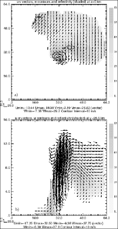
Figure 5. Wind vectors, vertical velocity (contours) retrieved from data sampled by two Doppler radars (see Fig.2) using the variational analysis method at iteration number 200. The location of cross-sections and plotting convections are the same as in Fig.4.
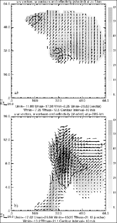
Figure 6. As in Figure 5, but for experiment NOWC, which excludes the mass-continuity weak constraint.

Figure 7. As in Figure 5, but for experiment NOSM, which excludes the smoothing terms in the cost function.

Figure 8. As in Figure 5, but for an experiment that does not include background (rawinsonde) data. The fields in the entire analysis domain are shown.

Figure 9. Same as Figure 5, except that the analyzed fields are shown for the entire analysis domain.
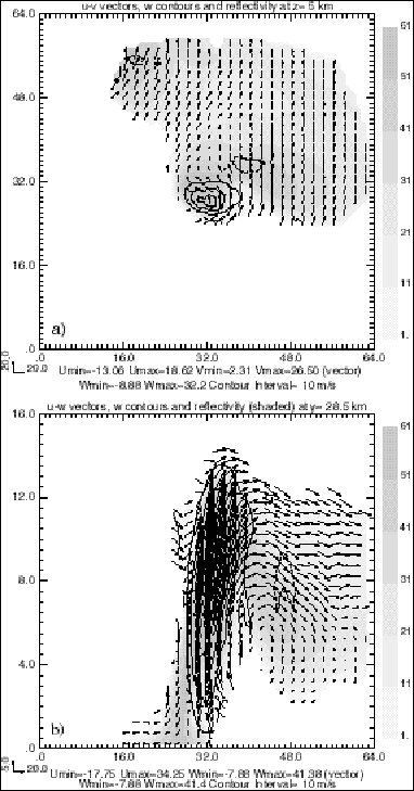
Figure 10. Same as Figure 5, but for experiment ERR1, which includes random observational errors up to 20 percent of the original values.
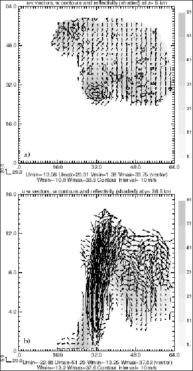
Figure 11. Same as Figure 5, but for experiment ERR3, which includes random observational errors up to 100 percent of the original values.
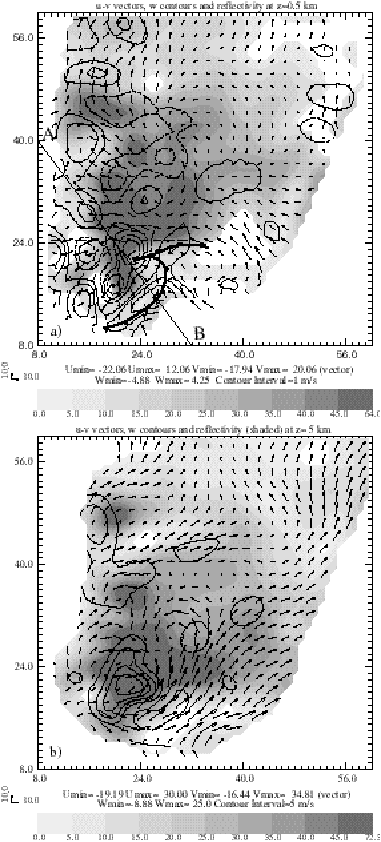
Figure 12. Wind vectors, vertical velocity (contours) retrieved using the variational analysis method for Arcadia, OK 17 May 1981 tornadic storm. a) Horizontal cross-section at z = 0.5 km. b) Horizontal cross-section at z = 5 km. c) Vertical cross-section through line A-B in panel a).
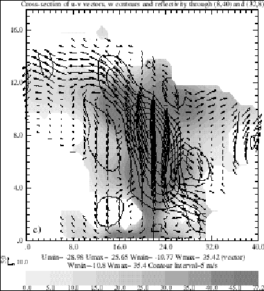
Figure 12. Continued. c) Vertical cross-section through line A-B in panel a).